How do we assess drained organic land when soil data simply does not exist? We know where the ditches are. We can see what the landscape looks like. But we do not know exactly where the organic soil is, or where drainage has actually altered the water regime enough that previously wet ground has now become dry.

We can and are allowed to use a defined proxy method to assess the extent, and rather report on the probability that land is drained, instead of assigning the label “disturbed wetland” to all land within a fixed 200 m Euclidean distance from the centreline of every ditch.

The IPCC accepts local variables and landscape analysis when soil and/or water table data are unavailable. The condition is that the methodology must be transparent and accompanied by an uncertainty assessment (IPCC, 2003, bls. 3.14–3.28; IPCC, 2006, Vol. 4, Ch. 2, bls. 2.8–2.12). In the 2006 guidelines, the definition of drained organic soils appears to rest mainly on a lowering of the water table  that is, a changed water regime  not on whether ditches have been dug (IPCC, 2006, Vol. 4, Ch. 4, bls. 4.1–4.5). This distinction could matter a great deal. It is not enough to have dug a ditch; the water must have had a clear path to drain away, causing a permanent change in the water regime.

Analysis and technical explanation

Several Nordic countries have reported on disturbed wetlands and their extent by looking at more factors than ditch excavation alone. Finland, for example, bases its assessment of drained land on the interplay of soil data, ditch networks, and elevation models, where hydrological context is included in the analysis (Finnish Environment Institute, 2022, bls. 156–178). Germany uses elevation and flow models to define active drainage in peatlands instead of a fixed distance from ditches (UBA, 2021, bls. 421–429). The Netherlands assesses the extent of drained areas through extensive water management, allowing them to report on actual runoff rather than merely inferring it from the presence of dug ditches (Arets o.fl., 2020, bls. 89–94).

What these countries have in common is that the assessment of disturbed wetland extent is more about evaluating the water regime than simply counting ditches and their total length. Their analysis examines how geographic location affects the water table, based among other things on the connection of the ditch network to streams and rivers, slope, flow and elevation models, sinks and sources, and related factors.

We can and should approach this in a comparable way, and we ought to look into it as soon as possible.

Prerequisites for a proxy approach

We propose that the assessment of disturbed wetland should rest on four main prerequisites. All four must be met for an area to be classified as disturbed wetland.

1. Land use in the area is capable of lowering the water table (e.g. ditch excavation).
2. The landscape and surface must meet certain conditions that confirm water could have accumulated and formed wetland  meaning the area was actually wetland before.
3. Surface slope. We have used a threshold of ≥10° overall. Water does not accumulate where it runs away.
4. Water must be able to drain off or away from the area. This is probably the single most important factor. If the water cannot get away, we may need to distinguish between active drainage on the one hand and the mere impact of ditch digging on the other.

Ditch density instead of a fixed distance

The ditch network is the direct cause and therefore carries the most weight. But instead of drawing a 200 m buffer from the centreline of every ditch, we first look at ditch density  linear metres per hectare, or m/m². This approach reflects the idea that drained land should be seen as a systemic change in water regime rather than a localised phenomenon. Where a high number of ditches and total linear metres  that is, high density  are present, their zones of influence overlap.

On flat land with a dense ditch network, the groundwater table can therefore drop far beyond any single ditch line. Research on drained land shows that the zone of influence of ditches depends on their density, their connections, and their position in the landscape. Ditches can reach hundreds of metres on gentle slopes over a small area (Holden o.fl., 2004, bls. 104–108; Joosten & Clarke, 2002, bls. 92–98). Density is therefore a better approach for assessing the actual change in water regime and extent of drained land than a simple buffer.

Saturation analysis

Instead of choosing a single distance (e.g. 200 m), the area is assessed based on ditch density, but we need to examine what happens at incrementally increasing distances. For example, we would look at a 25 m radius (5×5 = 25 m² pixels), then 50 m, 100 m, 200 m, 300 m, 400 m, and 500 m. For each radius, we report total linear metres and the number of ditches. The change between steps can and will show that, despite increasing linear metres of ditches per unit area, the total affected area stops growing at certain intervals.

This is how we identify where saturation occurs. Saturation appears when increasing the radius produces only marginal additional area of drained land. We can interpret this as the ditch network’s zone of influence having reached its true extent in that area.

If, for instance, going from 200 m to 300 m yields a substantial increase in area, but going from 300 m to 400 m yields very little change, this suggests that the actual zone of influence lies closer to 300 m than to 200 m. Such a saturation analysis makes it possible to choose a radius on a geographic and well-reasoned basis.

This saturation analysis is fully consistent with the Good Practice Guidelines, which recommend that member states carry out sensitivity analysis when results depend on key assumptions such as these (IPCC, 2003, bls. 6.2–6.18). When density and sensitivity analysis can demonstrate how the area changes with radius and where stability is reached, the method is both transparent and well defensible in the carbon accounting.

The meaning of the saturation analysis is twofold. First, it reduces the risk of systematic underestimation (if the radius is too small) or overestimation (if the radius is too large). Second, it strengthens our professional basis for assessing the extent of disturbed wetland. We will be able to show that the choice of ditch influence zones now rests on measurable, systematic factors rather than a “best guess” based on a handful of measurements.

In other words, saturation becomes not only geographic and verifiable, but an indicator of actual change in the water regime and the spatial extent of ditch influence.

Note that saturation is not the same as drained land.

Integrating the main factors

To assess the extent of drained land, we need all four main factors. We need to think of this as a logical, stepwise process where we move from landscape prerequisites to probability assessment and finally to area calculation. We are not measuring drainage directly  we are inferring it from hydrological and geographic factors.

We start with the ditch network, the direct cause of drainage. Instead of drawing a fixed distance  say a 200 m buffer around every ditch  we assess how dense the ditch network is across the landscape. Density is calculated as the length of ditches within a given radius, expressed as linear metres per hectare or square metre.

Next we take the landscape into account. Depressions tell us whether an area lies lower than surrounding land and therefore had a higher likelihood of having been wetland before drainage took place. Slope then excludes steep areas where it is unlikely that water accumulated. Flow analysis and connections to other ditches, lakes, rivers, and streams then ensure that we can identify areas where the water actually drains away  because without a connection to a discharge system, it is doubtful that the water regime has been permanently altered.

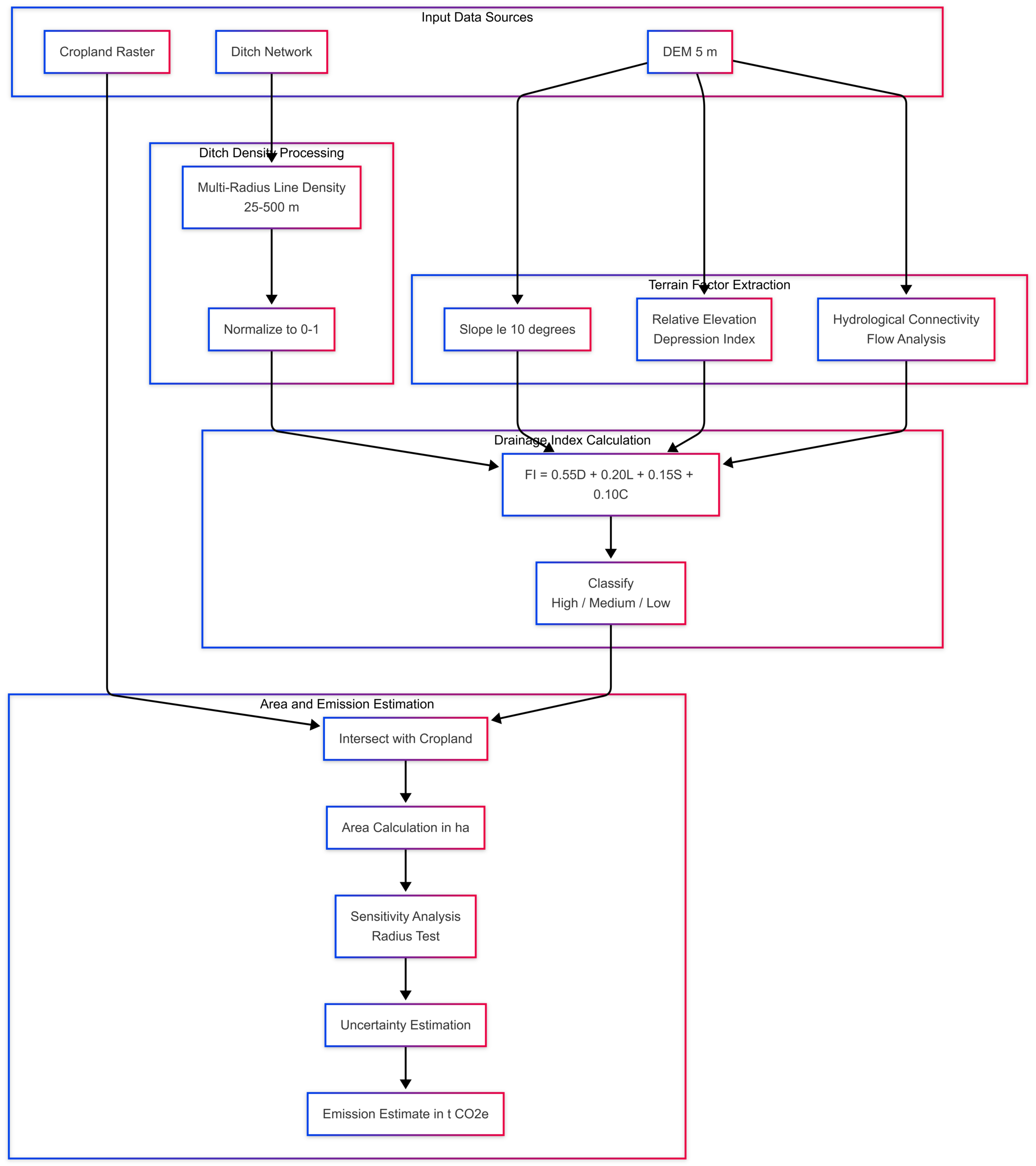
These four main factors  (1) ditch density, (2) depressions and elevation/DEM, (3) slope, and (4) water connectivity  are then combined into a single drainage index (if you have a better name, please suggest one). It ranges from 0 to 1, where a higher value indicates a greater probability of actual drainage. Each pixel receives its own index value.

We then choose a threshold  for example 0.7  and classify all pixels ≥ 0.7 as likely drained. This is a methodological decision that needs to be justified and tested with sensitivity analysis.

Finally, we examine the overlap of the result (the raster layer with the drainage index) against cropland. The overlap shows the geographic location and number of intersecting pixels  areas that in all likelihood sit on organic soil and are drained accordingly. The area is calculated simply by counting the pixels that meet two conditions: they are above the threshold we chose and they overlap with cropland. The total gives us geographically distinguishable areas reporting organic soil within cropland.

The extent of drained land is therefore the outcome of: a correct choice of scale (through saturation analysis), a reasonably well-defined flow model (D, L, S, C) that is further constrained by land use. This is not one analysis, or one measurement with one variable  it is an integrated inference built on the best available data. The inference then demonstrates, in a measurable way, a certain causal relationship in the landscape with and without human intervention.

Conclusion

We want to carry out a proxy assessment and explore landscape analysis using these four main factors  ditch density, elevation model, slope, and water connectivity  instead of a 200 m distance from ditches. Saturation analysis shows us where the real influence of the ditch network extends to. This is consistent with IPCC guidelines on proxy methods and sensitivity analysis when soil data are missing.

Arets, E. J. M. M., van der Kolk, J. W. H., Hengeveld, G. M., Lesschen, J. P., Kramer, H., Kuikman, P. J., & Schelhaas, M. J. (2020). Greenhouse gas reporting of the LULUCF sector in the Netherlands. Wageningen Environmental Research.

Finnish Environment Institute. (2022). National Inventory Report Finland 1990–2020: LULUCF sector.

Holden, J., Chapman, P. J., & Labadz, J. C. (2004). Artificial drainage of peatlands: Hydrological and hydrochemical process implications. Progress in Physical Geography, 28(1), 95–123.

Intergovernmental Panel on Climate Change (IPCC). (2003). Good Practice Guidance for Land Use, Land-Use Change and Forestry. IGES.

Intergovernmental Panel on Climate Change (IPCC). (2006). 2006 IPCC Guidelines for National Greenhouse Gas Inventories. Volume 4: Agriculture, Forestry and Other Land Use. IGES.

Joosten, H., & Clarke, D. (2002). Wise use of mires and peatlands. International Mire Conservation Group.

Umweltbundesamt (UBA). (2021). National Inventory Report for the German Greenhouse Gas Inventory 1990–2019. Federal Environment Agency, Germany.

Tilgangurinn með þessum index er að reyna að meta flatarmál áhrifasvæða skurða, með því að leggjs saman fjóra landfræðilega meginþætti í landslaginu. D, L, S og C

Aðferðin sem notuð hefur verið hingað til er að búa til 200m buffer (jaðar) út frá skurðum til beggja átta, draga svo frá þau tiltæku landfræðilegu gögn sem við gerum ráð fyrir að geti skorið úr um að á þessari staðsetningu  hafi aldrei verið lífrænn jarðvegur, t.d halli, melar, sandar, hraun os.frv.

Þetta er einföld nálgun og auðvelt að útskýra hana.

Mögulega allt of einföld?

(Four Inputs= FI)

Hér er lögð til önnur aðferð sem byggir á svokölluðum framræsluvísi eða drainage index.

FI = 0.55 * D + 0.20 * L + 0.15 * S + 0.10 * C = 0-1

1. Skurðaþéttleiki (55% vægi). Því fleiri lengarmetrar skurða per/m² því meiri eru áhrifin
2. Hæðarlega (20% vægi). Vatn safnast saman í lægðum.
3. Halli (15% vægi). Hallagreining, því brattara því líklegra er að vatn renni af svæði og eða renni ekki neitt frá flatari svæðum.
4. Flæðigreining. (10% vægi) Skurðir þurfa að tengjast öðrum skurðum og eða vatnsföllum og enda svo á því að skila því vatni sem inn á það hefur runnið, út aftur.

(Four Inputs) er þá FI = 0.55 * D + 0.20 * L + 0.15 * S + 0.10 * C = 0-1 gildi á hverja myndeiningu. Niðurstaðan geta verið gildin 0.10, 0.40 og eða 0.70. Því lægra gildi því meiri líkur eru á að um raskað land sé að ræða, Hver myndeining er 5X5m og við værum því í öllum tilfellum að meta 25m² í einu.

Vísirinn býr þannig til grunnlag/þekju (Raster GRIDD) þar sem sumar myndeiningar eru líklegri til að vera framræstar og aðrar ekki, jafnvel þótt þær séu jafn langt frá skurði/um.

Jaðar greining (Multible Buffer Analysis).

Jaðarinn eða jaðrarnir eru búnir til í nokkrum fjarlægðum út frá skurðum þ.e 25m, 50m allt að 500m. Hann þjónar hér fyrst og fremst sem mælitæki, og þá á hversu margar myndeiningar (flatarmál) hafa það lág gildi að meta megi sem svo, jafnvel með ákveðinni vissu að þær hafi og séu að verða fyrir áhrifum skurða?

Fyrsti jaðarinn 25m ætti að innihalda margar myndeiningar með vísitölu sem greinir frá röskuðu svæði, eftir því sem fjarlægðin eykst því hærri er vísitalan og að lokum, mettun, þ.e gildi per/myndeiningu er alltaf 1. Þannig er fjarlægðin hætt að segja okkur eitthvað.

Tökum eitt dæmi (mjög einfalt). 3 myndeiningar sem eru allar í 150m fjarlægð frá skurði.

Vísitölugreiningin sýnir að þrátt fyrir sömu fjarlægðina fáum við 3 ólíkar niðurstöður. 1/3 myndeiningum er í halla og tengist skurðinum (há vísitala). 2/3 fær lægra gildi, því hún er á flatlendi og tenging við skurð lítil. Sú þriðja fær mjög lágt gildi (lægstu vístöluna) af þeim þremur þar sem hún liggur í lægð og vatn safnast þar fyrir. Fjarlægðin er sú sama en niðurstöðurnar þrjár eru ólíkar.

Annað dæmi. Ímyndum okkur svæði með háum skurðaþéttleika. Ef við notum 200m buffer skarast hringirnir og að lokum verður nánast allt svæðið merkt framræst. Aðferðin getur ekki greint á milli misraskaðra svæða. Allt verður eins. Með index greiningunni er hægt að greina frá breytileika á milli myndeininga, því sumar myndeiningar fá lágt gildi ef t.d tenging við skurð er slök og/eða vatn safnast þar fyrir.

Þriðja dæmið. Hugsum okkur stórt svæði með fáum skurðum sem liggja langt hver frá öðrum. Með fixed buffer fást litlir blettir í kringum hvern skurð og ekkert þar á milli. Indexinn getur hins vegar sýnt að áhrifin ná jafnvel enn lengra en 200m þar sem landslag styður við slíkt, eða styttra þar sem það gerir það ekki. Sömu fjarlægðir frá skurðum per/myndeiningu geta þannig greint frá mismiklu flatarmáli (fjölda myndeininga + 25m²) allt eftir því hvernig landslagið er.

Flatarmál áhrifasvæða frá skurðum samanstendur því af fjölda myndeininga með hátt vísitölugildi. Þegar radíusinn (Bufferinn/Jaðarinn) stækkar þá bætist alltaf við flatarmál hans, stærðin á jaðrinum (flatarmál) hans skiptir hins vegar engu máli, jaðarinn er fyrst og fremst mælitæki á þann fjölda myndeininga sem bætast við með auknu flatarmáli jaðarsins. Fjöldi myndeininga mun þannig aukast sem tilheyra sama kerfi. Þegar við hættum að sjá breytingar á gildum myndeininga þá eru skurðir hættir að hafa áhrif og fjarlægðin hætt að skipta máli.

Hvað varðar mat á flatarmáli framræsts lands þá hef ég sannfæringu fyrir því að index-aðferðin sé betri. Hún velur aðeins þær myndeiningar sem raunverulega virðast verða fyrir áhrifum frá skurðum og sleppir þeim sem hafa þau ekki. 200m buffer er einfaldari, og auðvelt að skilja hvers vegna hann er notaður, en hann bæði ofmetur og vanmetur svæði, sérstaklega þar sem skurðir standa þétt og/eða landslag er mjög breytilegt.

Indexinn gæti hins vegar þurft að túlka á mismunandi vegu, allt eftir tíma og rúmi. Einnig hef ég ekki nokkra hugmynd um hvar mörkin eigi að liggja fyrir það sem telst „hátt” eða “lágt” gildi,

En ef markmiðið er að færast nær raunveruleikanum, þá er raunhæfara að nota indexinn. (þ.e ef ofangreint meikar sens fyrir fleirum en mér)